Forward Selection Regression and Backward Elimination Regression

February 2025

(Forward selection and backward elimination regression techniques are now part of SPC for Excel Version 7).

Regression techniques are used to help determine which predictor variables have a significant impact on a response variable. Regression is often used to model the process. There are various regression techniques that can be used. For example, you can use multiple linear regression that includes all the predictor variables in the model. You can also use stepwise regression that adds or removes predictor variables in an iterative process.

This publication compares two stepwise iterative regression techniques: forward selection and backward elimination. The objective of each technique is to build a model based on the predictor variables.

In this issue:

• Introduction
• Example Data
• Forward Selection Regression
• Backward Elimination Regression
• Comparison of the Two Techniques
• Criticism of the Two Techniques
• Summary
• Quick Links

Please feel free to leave a comment at the end of the publication.  You can download a pdf copy of this publication at this link.

Introduction

Forward selection and backward elimination are both stepwise selection techniques to, hopefully, identify the most significant predictor variables to model a process. But they are quite different in their approach. Forward selection begins with an empty model. There are no predictor variables in the model. Each predictor variable is added to the model, one at a time. The predictor variable that provides the most improvement to the model, based on a given criteria such as the p-value, is added. This interactive process continues until there are no more predictor variables that can be added to the model based on the criteria.

Backward elimination, on the other hand, begins with all the predictor variables in the model. The predictor variable that meets the criteria (for example, largest p-value) is removed from the model. The regression is then run again and the next predictor variable meeting the criteria is removed. This continues until none of the remaining predictor variables in the model meet the criteria to be removed.

These two techniques are explained in more detail below using the same example data. This will help compare the results from the two techniques.  You can also view our previous articles on regression and stepwise regression at this link.

Example Data

Suppose we have seven predictor variables that we think might influence our response variable (y). We will use forward selection and backward elimination to build a model based on this data. The data are shown in Table 1.

Table 1: Example Data

Forward Selection Regression

Forward selection begins with an empty model. You must decide on the criteria for adding a predictor variable to the model. We will use the p-value and set the threshold to add a predictor variable to the model to be 0.25.  This means that a predictor variable must have a p-value less than 0.25 to be considered as a candidate to add to the model. The steps in forward selection are given below.

1. Begin with no predictor variables in the model.
2. Calculate the p-values for each individual predictor variable in the model.
3. Add the predictor variable with the lowest p-value to the model as long as it is below the threshold of 0.25.
4. After adding the predictor variable, re-evaluate the remaining predictor variables with the first predictor variable in the model.
5. Add the remaining predictor variable with the lowest p-value to the model as long as it is below the threshold of 0.25.
6. Continue until none of the remaining predictor variables have p-values less than the threshold.

Let’s apply the forward selection technique to the data in Table 1. The analysis below was done using the SPC for Excel software. The SPC for Excel software performs all the calculations automatically. We will go through each step that SPC for Excel does for you below.

You start with the empty model and regress Y on each predictor variable. This simply means running the regression for each predictor variable alone versus Y. Then, the predictor variable with the lowest p value is added to the model (as long as the p-value is less than 0.25). X4 had the lowest p value so it is added to the model in the first step. The results are given below.

Step 1: Added X4 to the Model

“Coeff.” is the coefficient of the predictor variable. The model at this point is:

y  = 6.133 – 0.00583*X4.

To compare the models, we will use R². R² measures the amount of variation in the model that is explained by the predictor variables. R² varies between 0 and 1, the closer to one the better the fit. R² for the model after step 1 is 66%. So, 66% of the variation in the response variable is explained by the model from Step 1.

The second step is then to include each predictor variable (one at a time) in the model that includes X4 and run the regression. Again, you select the predictor variable with the lowest p-value (and is below 0.25) and add that to the model. In this case, it was X3. The results for the second step are shown below.

Step 2: Added X3 to the Model

R² for this model is 77%. Adding X3 to the model increase R² from 66% to 77%.

You continue the process until none of the remaining predictor variables are less than 0.25.

Step 3: Added X1 to the Model

R² for this model is 91%.

Step 4: Added X2 to the Model 

R² for this model is 92%. Note that the p-value for X4 is now larger than the threshold. You do not remove it though. Once it is added to the model, it is not removed regardless of what happens to its p-value.

Step 5: Added X5 to the Model

R² for this model is 93%. The remaining predictor variables (X6 and X7) have p-values greater than the threshold, so no more predictor variables are added to the model. The finished model is:

y = 5.487 – 0.322(X1) – 0.002(X2) + 0.93(X3) – 0.001(X4) – 0.024(X5)

Backward Elimination Regression

Backward elimination begins with all the predictor variables in the model. You must decide on the criteria for removing a predictor variable from the model. We will use the p-value and set the threshold to remove a predictor variable from the model to be 0.10.  This means that a predictor variable must have a p-value greater than 0.10 to be considered as a candidate to remove from the model. The steps in backward elimination are given below.

1. Begin with all predictor variables in the model.
2. Run the regression with all predictor variables in the model.
3. Remove the predictor variable with the largest p-value (as long as it is larger than 0.10, the threshold value).
4. Run the regression with the remaining predictor values.
5. Remove the predictor variable with the largest p-value (as long as it is larger than 0.10, the threshold value).
6. Continue this process until there are no more predictor variables to remove from the model (all have a p-value less than 0.10).

We will now examine the data in Table 1 using the backward elimination in SPC for Excel, which goes through all the calculations automatically for you. We break it down by steps here.

You begin by running the regression with all predictor variables in the model. The major results are shown below.

Step 1: Run Regression with all Predictor Variables

R² for this model is 93%. The largest p-value is 0.9477 for X6. So, since it is larger than the 0.10 threshold, the next step is to remove X6 from the model and re-run the regression with the remaining predictor variables.

Step 2: X6 Removed from the Regression

R² for this model is 93%. X4 has the largest p-value and is still over the threshold, so it is removed next from the model.

Step 3: X4 Removed from the Regression

R² for this model remains at 93%. X7 has the largest p-value and is still over the threshold, so it is removed next from the model.

Step 4: X7 Removed from the Regression

R² for this model remains at 93%. X5 has the largest p-value and is still over the threshold, so it is removed next from the model.

Step 5: X5 Removed from the Regression

R² for this model is 92%. There are no more remaining predictor variables in the model that are more than the threshold of 0.10. The process ends here, and this is the final model:

y = 5.397 – 0.349(X1) – 0.002(X2) + 0.955(X3)

Comparison of the Two Techniques

The two techniques generated two different models.

Forward Selection: y = 5.487 – 0.322(X1) – 0.002(X2) + 0.93(X3) – 0.001(X4) – 0.024(X5)

Backward Elimination: y = 5.397 – 0.349(X1) – 0.002(X2) + 0.955(X3)

There are five predictor variables remaining in the forward selection technique compared to three predictor variables in the backward elimination technique. Despite this difference, both models reflect the actual results very well. Table 2 shows the values of y for the data in Table 1 for the backward elimination, forward selection, and the actual values.

Table 2: Comparison of Backward Elimination, Forward Selection and Actual Values

Figure 1 shows a graphical picture of the data in Table 2.

Figure 1: Comparison of Backward Elimination, Forward Selection and Actual Values

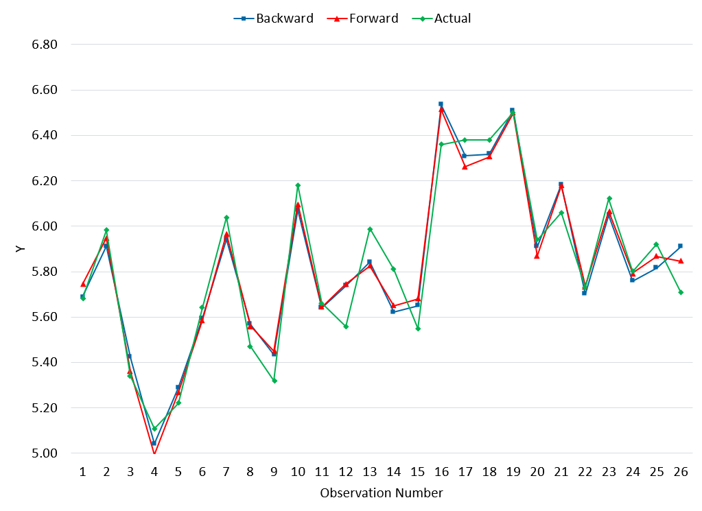
It appears from this data that both models fit the actual data well.

Criticism of the Two Techniques

It should be noted that there are those who do not think backward elimination or forward selection should be used. The issue revolves around the model selection which influences the p-values during the regression. We used 0.25 and 0.10 for the thresholds above, but these are somewhat arbitrary – and they do influence what predictor variables end up in the model. This selection bias can lead to incorrect p-values, biased coefficients, underestimated standard errors and overfitting of the model.

As with any model, it needs to be checked for how well it fits the original data but also how well it fits with new data that is generated.

Summary

This publication introduced two regression techniques: forward selection and backward elimination. Both are stepwise iterative processes that add a predictor variable to a model (forward selection) or that removes a predictor variable from a model (backward elimination). Both techniques end when there are no more predictor variables that meet the threshold.