Type 1 Gage Study

June 2024

Why do we measure things? We measure because we want to know where we are. Are things improving? Are they getting worse? Are they staying the same? To measure something, we need measurement systems. We want those measurement systems to be accurate and precise; to be able to tell the difference between samples; and to tell if the sample is within specification.

We need proof that our measurement systems can do these things. How do we get this proof? We have to study the variation in our measurement system. We do that by conducting different gage studies.

It is often recommended that you begin studying a measurement system by conducting a Type 1 gage study. This focuses your initial attention on the measurement device (e.g., gage) itself and not on any other sources of variation. A Type 1 gage study examines the repeatability and bias of a measurement device. This publication introduces the Type 1 gage study.

In this publication:

• Introduction
• Example Data
• Statistics Used in Type 1 Gage Study
• Run Chart in Type 1 Gage Study
• Bias in Type 1 Gage Study
• Capability Assessment (Cg and Cgk)
• Conclusion
• Summary
• Quick Links

Please feel free to leave a comment at the end of this publication.  You can download a pdf copy of this publication at this link.

Introduction

There is a new measurement device we are considering using. We want to do the initial study of this device by conducting a Type 1 gage study. A Type 1 gage study evaluates the repeatability and bias of a device. This is done by having one operator measure a known reference sample multiple times.

The repeatability and bias can then be evaluated by comparing the measurements to the reference value. This procedure also allows you to compare the variation in the measurement device to the tolerance to ensure the variation in the measurement device is not too large. You are essentially measuring the capability of the measurement device with a Type 1gage study.

To conduct the Type 1 gage study, you do the following steps:

1. Collect the data from one operator running the reference sample multiple times.
2. Calculate the statistics from the data
3. Construct a run chart to visually see the results
4. Determine if bias is present
5. Determine the measurement devise capability (Cg and Cgk)

You want to run the reference sample as many times as possible. It is recommended to run it 50 times.

Example Data

To conduct a Type 1 gage study, you need a reference sample. For our example data, we have a reference sample with a value of 12.306. One operator measures the reference sample 50 times using the measurement device. The results are shown in Table 1.

Table 1: Repeat Measurements on Reference Sample

What does the data in Table 1 represent? Since it the same reference sample being run by the same operator in the same measurement device, it represents how repeatable the measurement device is.

We will use this data to conduct the Type 1 gage study below. The upper specification limit (USL) for the process is 12.335. The lower specification limit (LSL) is 12.285. We start the analysis by calculating some statistics from Table 1.

Statistics Used in Type1 Gage Study

We will use the output from the SPC for Excel software for our analysis. The statistics are given in the table below.

Table 2: Statistic for Type 1 Gage Study

The average and standard deviation are calculated as usual. The study variation (SV) is k times the standard deviation. This measures the repeatability of the measurement device. The recommended value for k is usually 6. So, the study variation:

ks = 6(0.00485)= 0.0291.

If you use k = 6, then 99.73% of the measurements will fall within the range of ≠3s of the average.

The tolerance is USL – LSL. In this example, the tolerance is then:

Tolerance = 12.335 – 12.285 = 0.05.

At this point you can have a picture of how the study variation does against the tolerance. Figure 1 shows a histogram of the results in Table1 vs the specifications.

Figure 1: Study Variation vs Tolerance in Type 1 Gage R&R

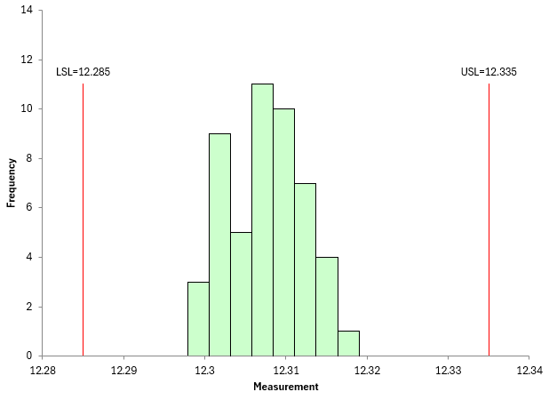
The histogram represents the repeatability of the measurement device – the results of running the reference sample over and over. You want the study variation to be within the spec limits (or the tolerance). The less room the study variation takes up compared to the tolerance the better. If the study variation gets too large to the tolerance, then the measurement device will have too much variation for its use.

One decision you have to make is how much of the tolerance that you can afford to be taken up by the study variation. The recommended value is 20%. We will denote this % by P. We will use 20% as P to calculate the gage capability indices (Cg and Cgk) and to use on the run chart.

MI in Table 2 represents the measurement increment. In this example, as shown by the data in Table 1, MI is 0.0001. Each value is measured to the nearest 0.0001. The MI as % of tolerance is then 0.0001/.05 = 0.20%. It is recommended that the MI as % of tolerance be less than 5%. So, this looks good for the measurement device.

The next step in a Type 1 gage study is to create a run chart to show how the results vary with respect to the reference value and the tolerance.

Run Chart for Type 1 Gage Study

The run chart for the data in Table 1 is shown in Figure 2 below.

Figure 2: Run Chart for Type 1 Gage Study

This chart plots each result from Table 2 in run order. The average (12.3075) is plotted. The reference value (12.306) for the sample is also plotted. The two red lines represent the tolerance band: the reference ± 0.1 times the tolerance.  Mathematically, this is:

Reference – (P/200)(Tolerance) to Reference + (P/200)(Tolerance)

12.306 – (20/200)(0.05) to 12.306 + (20/200)(0.05)

12.301 to 12.311

The tolerance band in Figure 2 is 12.311 – 12.301= 0.01. You can also calculate the tolerance band as the following:

Tolerance Band = (P/100)(Tolerance) = (20/100)(.05) = .01

The width between the two red lines represents 20% of the tolerance. If we had selected 50% as P, the two red lines would be the reference ± 0.25 times the tolerance.

If the measurement device is good, i.e., capable, all the results should be within those two red lines. That is not the case here. In fact, the following is true:

• There are 16 points outside the tolerance band.

The measurement system is not capable of producing results within the tolerance band. It doesn’t look good for the measurement device. There is too much variation. The next step is to determine if there is significant bias in the results.

Bias in a Type 1 Gage R&R

If the measurement device is accurate, we would expect the average of the repeat measurements on the reference sample to be the same as the reference sample’s true value, 12.306 in this example. Compare the average and reference lines in Figure 2. They are not the same. We would not expect them to be identical because of variation. The question we want to answer here is the following:

Is the difference between the average and reference value statistically significant?

This difference is called the bias and is a measure of how accurate the measurement device is. The bias is given by:

Bias = 12.3075 – 12.306 = 0.0015

The question is whether this is close enough to be zero, so there is no bias. We use a one-sample t test and p-value to determine this. You start by calculating the following t-statistic:

where N = number of test results and s = the standard deviation of the test results. The value of t is then:

Now, we calculate the p-value that defines the probability of getting this t-statistic if there is no bias. Our null hypothesis is that the bias is zero. We want to know what the probability of getting a t-statistic = 2.185 is if there is truly no bias. If the p-value is small (<=0.05 usually), we conclude that the probability of getting that value is low and accept that the bias is not zero.

You can use the Excel function TDIST to determine the p value.

p-value = TDIST(t, N-1, 2) = TDIST(2.185, 49, 2) = 0.0337

This p-value is small, which means that the probability of getting that t-statistic if there is no bias is small – not very likely. So, we conclude there is bias in the results. And since the bias is positive, we conclude that the measurement device tends to measure the reference sample on the high side. More bad news for the measurement device.

The next step is to assess the capability of the measurement device.

Capability Assessment (Cg and Cgk)         

There are two terms that are used to assess the capability of measurement devices in Type 1 gage studies: Cg and Cgk. We will start with Cg.

Cg

Cg is the ratio of the tolerance band to the study variation:

Cg = Tolerance Band/Study Variation = 0.01/0.0291 = 0.343

Cg is comparing the tolerance to the 50 results obtained by the operator. You want larger Cg values. If Cg = 1.33, about 75% of the study variation will fit into the tolerance band (P). If Cg is less than 1.33, the measurement device cannot measure the results accurately. More bad news for the measurement device with Cg = 0.343, but not surprising based on the previous results.

Another term associated with Cg is % Variability (repeatability). It is the ratio of the study variation to the tolerance. The smaller this ratio the better. 15% or less is usually desired. The % Variability (repeatability) for our measurement device is:

% Variability (repeatability) = Study Variation/Tolerance = .0291/0.05 = 58.2

This is also given by P/Cg. But it is greater than 15. Another mark against the measurement device.

Cgk

Cgk adds bias into the Cg calculation. It compares the tolerance with the total of the bias and the measurement variation. It is given by the following:                                                                    

Cgk = ((P/200)*Tolerance-|Bias|)/(SV/2)

Cgk = ((20/200)*0.05-|0.0015|)/(0.0291/2)

Cgk = 0.240

Since Cgk < 1.33, the measurement system capability is not acceptable.

The last parameter we will consider is the % Variability(repeatability + bias). This compares the measurement device repeatability and bias to the tolerance. The desired value is less than 15%. It is given by:

%Var (Repeatability + Bias) = P/Cgk = 20/0.240= 83.22

Since this Variability is greater than 15%, the measurement variation is too large.

Another mark against the measurement device.

Conclusions

It is clear from the results that this measurement device is not fit for our purposes. The study variation to tolerance is too large, there is bias present and the capabilities Cg and Cgk are too small. There is no reason to go on to the Gage R&R studies.

Summary

This publication introduced the Type 1 gage study. This is the first step in beginning to analyze how good a measurement device is and should be done before going on to the Gage R&R studies. The Type 1 gage study compares the repeatability and bias of the measurement device to the tolerance. Two capability ratios, Cg and Cgk, were introduced. You want Cg and Cgk to be greater than 1.33