August 2024

You might think this sounds like simple linear regression. It is not. Both techniques compare one response variable (Y) to one predictor variable (X). In simple linear regression, only Y has measurement error. In Deming regression, both X and Y have measurement error. This makes Deming regression a great technique for comparing two measurement methods. Both have measurement error.
In This Issue:
- Overview of Deming Regression
- Example
- Determining the Measurement Errors for X and Y
- Calculating Lambda
- Collecting the Data for Deming Regression
- Performing the Regression
- Deming Regression Output
- Summary
- Quick Links
Please feel free to leave a comment at the bottom of the publication. You can download a pdf copy of this publication at this link.
Overview of Deming Regression
Deming regression is a technique used to fit a straight line to two continuous variables, where both variables, X and Y, are measured with error. It is often used to compare measurement methods. It is used with paired measurements (xi and yi) and associated error (s and t):
xi = Xi + si
yi = Yi + ti
The equation that Deming regression fits is:
Y’i = bo + b1X’i
where bo and b1 are the intercept and slope coefficient , and X’i and Y’i are the estimates of the true values of Yi and Xi.
The first step is to ensure that the two test methods are in statistical control. When this is true, you can estimate the measurement error associated with both test methods. This allows you to estimate lambda which is the ratio of the measurement system variances. Then you can run the Deming regression to calculate the coefficients in the above equation and use various statistical tests to see if the two methods give similar results.
Example
Suppose you and one of your suppliers have the “same” test method for determining a key quality characteristic of a part. You want to determine if the two test methods are comparable and want to use Deming regression to determine if the two methods are comparable. To do this, you know you will need to determine estimates of the measurement error for each test method. After that, you will take 30 parts and test them in each test method. The tests are nondestructive. Then you will run the Deming regression and reach a conclusion about whether the two test methods are comparable or not.
For this article, the supplier will be Test 1 and represented by X. You (the customer) will be Test 2 and represented by Y. Let’s walk through how this happens with Deming regression.
Determining the Measurement Errors for X and Y
To run the Deming regression, you need estimates of the measurement errors for each of the two tests. You can get these estimates from Gage R&R studies you have done on the tests. If you don’t have measurement error estimates from the past Gage R&R studies, I recommend you use the EMP consistency study. This is one of Dr. Donald Wheeler’s Evaluating the Measurement Process techniques. Part of that analysis involves constructing an individuals (X-mR) control chart from repeated measurements by one operator on one part. If the moving range chart is in statistical control, you can estimate the measurement error. Table 1 shows the repeated measurements for Test 1 (the X values from your supplier) for one part.
Table 1: Repeated Measurements Results for Test 1 (X)
| Sample No. | X | Sample No. | X | |
| 1 | 1.354 | 16 | 1.355 | |
| 2 | 1.351 | 17 | 1.354 | |
| 3 | 1.353 | 18 | 1.353 | |
| 4 | 1.355 | 19 | 1.351 | |
| 5 | 1.351 | 20 | 1.354 | |
| 6 | 1.350 | 21 | 1.355 | |
| 7 | 1.353 | 22 | 1.354 | |
| 8 | 1.354 | 23 | 1.353 | |
| 9 | 1.351 | 24 | 1.351 | |
| 10 | 1.354 | 25 | 1.352 | |
| 11 | 1.353 | 26 | 1.355 | |
| 12 | 1.351 | 27 | 1.354 | |
| 13 | 1.352 | 28 | 1.353 | |
| 14 | 1.351 | 29 | 1.354 | |
| 15 | 1.354 | 30 | 1.355 |
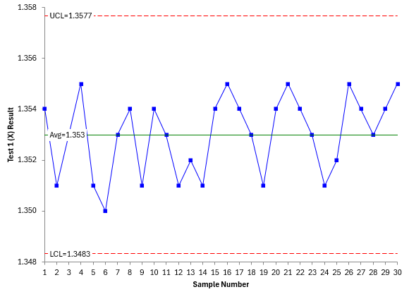
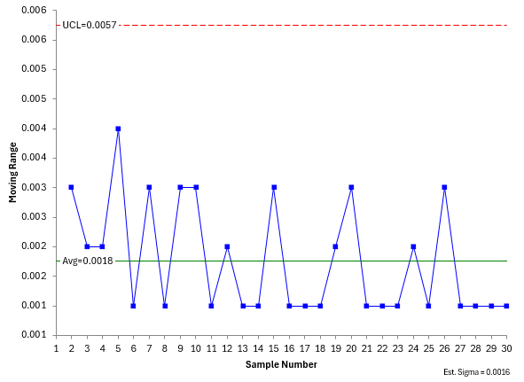
These 30 results are used to construct the individuals control chart. Please see our SPC Knowledge Base article for more information on how to construct and interpret individuals control chart. Figure 1 shows the X and mR chart for the Test 1 data.
Figure 1: X-mR Chart for Test 1 (X) Data
Since there are no points beyond the control limits nor any patterns in the two charts, both are said to be in statistical control. This test method is consistent and predictable. Please note this:
Before running the Deming regression, the two test methods must be in statistical control. If they are not, then you do not know what the methods will produce in the future.
This is often overlooked in doing tests like the Deming regression. Since the test is in statistical control, you can estimate the measurement error using the average moving range on the mR chart. The average range (R) is 0.0018. The measurement error (s) for Test 1 is then:
s = R/1.128 = 0.0018/1.128 = 0.0016
This process should be repeated for Test 2 – your test method. The data for the repeated measurements on a single part for Test 2 are shown in Table 2 below.
Table 2: Repeated Measurements Results for Test 2 (Y)
| Sample No. | Y | Sample No. | Y | |
| 1 | 1.350 | 16 | 1.350 | |
| 2 | 1.350 | 17 | 1.352 | |
| 3 | 1.356 | 18 | 1.350 | |
| 4 | 1.350 | 19 | 1.350 | |
| 5 | 1.350 | 20 | 1.350 | |
| 6 | 1.350 | 21 | 1.350 | |
| 7 | 1.350 | 22 | 1.356 | |
| 8 | 1.356 | 23 | 1.354 | |
| 9 | 1.356 | 24 | 1.354 | |
| 10 | 1.351 | 25 | 1.350 | |
| 11 | 1.350 | 26 | 1.350 | |
| 12 | 1.350 | 27 | 1.350 | |
| 13 | 1.356 | 28 | 1.354 | |
| 14 | 1.356 | 29 | 1.356 | |
| 15 | 1.355 | 30 | 1.350 |
You may construct the individuals control chart on the data in Table 2. We will not do that here to save some time and space. But Test 2 is in statistical control. The average moving range for Test 2 is 0.0022. The measurement error (t) for Test 2 is then:
t = R/1.128 = 0.0022/1.128 = 0.002
At this point, we have the two estimates of the measurement error for the tests and the knowledge that both tests are in statistical control. We can move forward with the Deming regression.
Calculating Lambda
Lambda (l) is the ratio of the measurement errors (as variances) between the two tests:
l = s2/t2
Note that the ratio is X (Test 1) to Y (Test 2). Some sources use the ratio of Y variance to X variance. The equations below involving lambda use the ratio as shown in the equation above, i.e., X to Y. This value is assumed constant in the Deming regression. For our two tests, the value of lambda is:
l = s2/t2 = (0.0016)2/0.002)2 = 0.64
Collecting the Data for Deming Regression
The next step is to collect the data for the Deming regression. Thirty parts that reflect the specification range are collected. Each part is numbered and run in each of the two tests (the supplier’s and the customer’s test). The results are shown in Table 3.
Table 3: Data for 30 Parts from Supplier (X) and Customer (Y)
| Part No. | X | Y | Part No. | X | Y | |
| 1 | 1.327 | 1.338 | 16 | 1.295 | 1.294 | |
| 2 | 1.296 | 1.306 | 17 | 1.381 | 1.375 | |
| 3 | 1.350 | 1.337 | 18 | 1.336 | 1.319 | |
| 4 | 1.299 | 1.312 | 19 | 1.368 | 1.382 | |
| 5 | 1.386 | 1.393 | 20 | 1.326 | 1.306 | |
| 6 | 1.388 | 1.393 | 21 | 1.351 | 1.363 | |
| 7 | 1.335 | 1.337 | 22 | 1.334 | 1.350 | |
| 8 | 1.337 | 1.331 | 23 | 1.368 | 1.369 | |
| 9 | 1.298 | 1.294 | 24 | 1.382 | 1.381 | |
| 10 | 1.352 | 1.350 | 25 | 1.362 | 1.370 | |
| 11 | 1.310 | 1.306 | 26 | 1.360 | 1.363 | |
| 12 | 1.308 | 1.313 | 27 | 1.344 | 1.357 | |
| 13 | 1.332 | 1.331 | 28 | 1.333 | 1.337 | |
| 14 | 1.385 | 1.381 | 29 | 1.315 | 1.319 | |
| 15 | 1.296 | 1.300 | 30 | 1.349 | 1.356 |
Performing the Regression
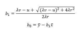
The following equations give the estimates of the coefficients that minimize the Deming regression sum of squares.
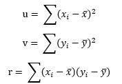
where b1 and bo are estimates of b1 and bo respectively, x and y are the means of yi and xi respectively, and
Using = 1.340 and = 1.342, the values for u, v, and r for the data in Table 3 are:
u = 0.0252587
v = 0.0272687
r = 0.0251167
With lambda = 0.64, the values of the coefficients are:
b0 = -0.0389
b1 = 1.031
The best fit equation is then given by:
y = -0.0389+ 1.031x
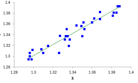
You can get an idea of how good the fit is by plotting Y vs X and the best-fit line. This is done in Figure 3.
Figure 3: Deming Regression Results
Figure 3 shows most of the points are near the best-fit line, so this would imply that there is a correlation between the two test methods. They give comparable results.
Deming Regression Output
In addition to the best-fit equation and Figure 3, there is other output that often accompanies Deming regression in software to help you analyze the results. We will look at the output from the SPC for Excel software which contains Deming regression.
|
Regression Coefficients |
|||||||
|
Coefficient |
Standard Error |
df |
t Stat |
p-value |
LCL |
UCL |
|
|
Intercept |
-0.0389 |
0.0652 |
29 |
-0.597 |
0.5552 |
-0.172 |
0.0944 |
|
X |
1.031 |
0.0484 |
29 |
21.31 |
0.0000 |
0.932 |
1.129 |
The table above contains information on the regression coefficients. The “Coefficient” column contains the values of b0 and b1 calculated above. The standard error is estimated using a jackknifing technique. This is a resampling method that is used to estimate the standard error of a statistic, in our case, the coefficients. The technique involves leaving out one observation at a time and calculating the values for each of these. The results can be used to estimate the standard errors.
The rest of the table is the typical regression coefficient table where:
- df: degrees of freedom, N – 1, where N is the number of parts in the study; some sources recommend using N- 2.
- t Stat: the t statistic given by coefficient/standard error (i.e., 1.031/.0484 = 21.31).
- p-value: the probability of getting that t statistic if the null hypothesis is true.
- LCL: the lower confidence limit.
- UCL: the upper confidence limit.
Let’s explore the p-value a little more. With the intercept (b0), we are testing two hypotheses:
H0: b0 = 0
H1: b0 ≠ 0
Ho is the null hypothesis; H1 is the alternative hypothesis. For the intercept, we calculated a t statistic (-0.597). The p-value represents the probability that we would get this value for the t statistic if the null hypothesis is true. If the p-value is sufficiently small (often, ≤ 0.05), we conclude that the probability of getting this t-statistic is small and the null hypothesis is rejected – the intercept is different than 0. If the p-value is larger, we conclude that the probability of getting this t-statistic is large and the null hypothesis is accepted. The intercept can equal 0.
The p-value for the intercept is 0.5552. Here, the p value is large, so we accept the null hypothesis and conclude the intercept could be 0.
The same approach is used for the coefficient. We are testing the null hypothesis that the coefficient is 0. The p-value for the coefficient is very small (0.0000). We conclude that we would not get this p-value if the null hypothesis is true, so we reject the null hypothesis and conclude that the coefficient is significantly different from 0.
The p-values can be calculated using the Excel function T.DIST.2T. The two entries are the absolute value of the t- statistic and the degrees of freedom.
Now, let’s explore the confidence limits a little more. The confidence limit for the intercept is -0.172 to 0.0944. Note that this confidence interval contains 0. This means that it is possible for the intercept to be 0. This matches what we concluded from the p-value. The confidence limit for the coefficient is 0.932 to1.129. Note that it does not include 0, so we conclude that the coefficient is significantly different from 0.
The confidence intervals are calculated as b +/- t(SE), where b is the intercept or coefficient, t is the t value and SE is the standard error for b. The t value can be calculated using Excel’s formula T.INV.2T, where the input is alpha value (usually 0.05), and the degrees of freedom.
So, Figure 3, along with the p-value and the confidence intervals imply that the two methods give comparable results.
You can also do hypothesis testing to directly test if the Deming regression slope is 1. The null hypothesis is that b1 = 1 and the alternate hypothesis is that b1 <> 1. The t test statistic in this case is:
t = (b1 – 1)/SE(b1)
Likewise, you can directly test that the two means, and, are the same. In this case, the test statistic is:
t = (y –x) /SE(y –x)
The output from the SPC for Excel program is given below for the hypothesis testing.
|
Hypothesis Testing |
|||||||
|
Parameter |
Standard Error |
df |
t Stat |
p-value |
LCL |
UCL |
|
|
Slope Test |
0.0305 |
0.0484 |
29 |
0.632 |
0.5326 |
-0.0838 |
0.145 |
|
Means Test |
0.00200 |
0.00162 |
29 |
1.232 |
0.2280 |
-0.00184 |
0.00584 |
You interpret this table the same way you did for the regression coefficients. The hypothesis tests for the slope are:
H0: b1 – 1 = 0
H1: b1 – 1 ≠ 0
Note that the slope test has a high p-value and the confidence limit contains 0. This means that b1 – 1 can be 0.
The null hypothesis for the means test is that the difference in the two means is 0; the alternate hypothesis is the difference in the two means is not 0. The means test has a high p-value as well and the confidence interval contains 0. So, you conclude that the means are the same.
The slope test and the mean test further confirm that the two methods are comparable. Note, that if either of these tests fail, the two methods are not comparable.
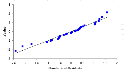
To further determine how good of a model the Deming regression produces is to see if the residuals are normally distributed. There are a number of ways of doing this. One option in the SPC for Excel program is to determine if the standardized residuals are normally distributed by doing a normal probability plot. Residuals are the difference between the actual values and the predicted values. The standardized residuals are the residuals divided by the standard deviation of the residuals. Figure 4 is a normal probability plot of the standardized residuals.
Figure 4: Normal Probability Plot of Standardized Residuals
If the points lay along the straight line, the residuals are normally distributed.
The conclusion for these two test methods is they produced comparable results.
Summary
This publication introduced Deming regression. This technique is used to determine if two test methods produce comparable results. You start by ensuring both test methods are consistent and predictable and use those results to determine the measurement error and set the value of lambda. You then run paired measurements through both tests and perform the Deming regression to estimate the coefficients as well as perform the hypothesis tests. The slope test and means test confirm if the two methods are comparable.
Very nice introduction to Deming’s regression.
However, the fact that we do not reject the null hypotheses intercept equal to zero and slope equal to 1 is not sufficient for concluding that the two measurement methods are in agreement. Indeed, the 95%CI of the slope (and intercept) are too wide. It is necessary to fix “a priori” two “agreement thresholds” (0.9 and 1.1 for example for the slope) and the conclusion of agreement is possible if the 95%CI are within these thresholds like an equivalence test.
Good point on setting what is an acceptable difference that the two methods are in agreement. I agree you need to add that to the process. You would have to use your knowledge the process to set those limits. You could run a paired equivalence test to see if the means are within an acceptable range. Thanks for the comment.
What about the The nonparametric Passing-Bablok procedure, which also compares two methods? Will this be incorporated in SPC for Excel?
I am not familiar with the Passing-Bablok procedure. I will look into it. Thanks.
The Passing – Bablok regression compares two methods by considering them in agreement if the 95%CI of the slope includes 1 and the intercept includes 0.
So, there is the problem I said before of 95% CI too wide deponing for a no agreement that wrongly allows to conclude for the agreement. Furthermore, the testing procedure in the agreement settings is an equivalence test and accordingly the required sample sizes have to be calculated. I think that the Passing and Bablok regression is a procedure that has to be forgot in an agreement analyis.
You can see my papers: Cesana Antonelli Ferraro Critical appraisal of the CLSI guideline EP09c 10.1515_clinical chemistry and laboratory medicine-2024-0595
Cesana Antonelli Sample_Size_for_Agreement_Studies_on_Quantitative variables_Epidemiology Biostatistics and Public Health 2024 for the sample size; paper correcting Shieh’s recent proposal.
Interesting article. I think this what Professor Peter Sprent (University of Dundee) called stochastic regression circa 1969.