Can the Rameriz-Runger Statistic Be Used as a Process Stability Index?

April 2024

Is your process in statistical control?  To find out, we have to construct a control chart and interpret it. Wouldn’t it be nice if there was just a single metric, one number, which would give us that answer. Over the years, there have been attempts to create a process stability index – a number that provides an answer to the question of whether your process is in statistical control or not.   

An easy process stability index is the ratio of the global standard deviation (s) to the within sigma (s) :

SI = Long Term Variation/Short Term Variation = s/s

But there are problems with that process stability index.  Dr. Donald Wheeler recently published an article that described the Rameriz-Runger statistic, which uses the above ratio.  His article examines the Rameriz-Runger statistic’s ability to determine if a dataset is homogeneous.  This would imply that it might be able to determine if a process is in statistical control – as an in control process implies that the data is homogeneous.  This publication takes a look at whether the Rameriz-Runger statistic can be an indicator of whether a process is in statistical control or not.  Two specific examples are provided to show the calculations.  Then simulations are run to determine the impact of using the Rameriz-Rungers statistic to judge if a process is in control or not.

In this publication:

• Introduction
• Process Capability Metrics
• A Process Stability Index
• The Rameriz-Runger Test Statistic
• “In Statistical Control” Example
• Out of Statistical Control Example
• The Simulations
• Summary
• Quick Links

Please feel free to leave a comment at the end of this publication.  You can also download a pdf copy of the publication at this link.

Introduction

How do you know if you are process is in statistical control?  Obviously, you make a control chart and interpret it.  But isn’t there an easier way?  Just one number to look at and say the process is in or out of statistical control?  Wouldn’t it be nice if that was true?  Tied closely to a process stability index is our process capability metrics.  We will start with a review of those metrics.

Process Capability Measures

Process capability measures (e.g.,  C_p and P_p) are intended to be measures of how well a process meets specifications.   Before calculating these measures, you should ensure that the process is consistent and predictable – in statistical control.  But quite often, people just rush to do the process capability analysis, without worrying about that issue of statistical control.  The calculations are easy to do.

The calculations for the C_p and C_pk capability indices are given below.  C_p is called the capability index while C_pk is the capability index taking into account where the process is centered.

C_p = (USL-LSL)/6σ

C_pk = Minimum (C_pu, C_pl)

C_pu=(USL-Average)/3σ

C_pl=(Average-LSL)/3σ

USL and LSL are the upper and lower specification limits, respectively.  The average is the average of all the results.  s is the estimated standard deviation from a range control chart.  If you are using an individuals control chart, then the estimated standard deviation is given by:

σ =  R̅/1.128

where R̅ is the average moving range between consecutive points on the moving range chart.

The calculations for the P_p and P_pk capability indices are given below.  P_p is called the performance index while P_pk is the performance index taking into account where the process is centered.

P_p=(USL-LSL)/6s

P_pk = Minimum (P_pu, P_pl)

P_pu=(USL-Average)/3s

P_pl=(Average-LSL)/3s

where s is the calculated standard deviation using all the data (e.g., using STDEV function in Excel).

Note that the only difference in these equations is the capability index uses sigma (σ) for the variation measure while the performance index uses the calculated standard deviation (s). Sigma (s) is often called the “short-term” variation.  s measures the global variation and  is often called the “long-term” variation.

So, the calculations are easy.  Put in the numbers and you have your process capability analysis done. But what about that issue of control?

There is still a way to “judge” if the process is in statistical control, even without constructing a control chart.  You can compare the two standard deviations used in the calculations above.  

If the two standard deviations are close to the same value, then the process is most likely in statistical control.  If the two standard deviations are not close, then the process is most  likely not in statistical control. For more details on this, please visit our SPC Knowledge Base article “What Do The Process Capability/Performance Metrics Measure?.”

A Process Stability Index

The description above says the two values of the standard deviation must be “close” for the process most likely to be in statistical control.  What is “close” in this situation?  When a process is in statistical control, it means that the short-term variation (s) is the same as the long-term variation (s).  A simple process stability index (SI) is then:

SI = Long Term Variation/Short Term Variation = s/s

If SI = 1 or is close to 1, then the short-term variation and the long-term variation are essentially the same and the process is probably in statistical control.  The further SI gets away from 1, the more likely the process is out of statistical control.

Note that SI is also the same as the ratio of C_p/P_p.

But we still have the same problem.  We now have a stability index, but still not a clear test if the process is in control or not.  We need a test that gives us more insight.  The Ramirez-Runger test is a possibility.

The Ramirez-Runger Statistic

In a recent paper, Dr. Donald Wheeler discussed a test you can use to determine the lack of homogeneity in a dataset.  His last sentence in the paper states:

“If you are not already starting your analysis with a process behavior chart, then the Ramirez-Runger test is the test to use before all other tests.”

We are assuming we are skipping that control chart at first, so Dr. Wheeler says to use the Ramirez-Runger statistic. 

The Rameriz-Runger statistic is given by:

Rameriz-Runger Statistic = (s/s)²

Note that this is simply the square of the stability index introduced above.  It means you are dealing with variances, not standard deviations. 

Again, values close to 1 would imply that the process is in statistical control.  But Dr. Wheeler shows that there is a test that determines if the statistic is extreme or not.   The statistic follows the F-distribution.  You can determine the p-value for the statistic by using the FDIST function in Excel.   

p-value = FDIST(Rameriz-Runger Statistic, df in numerator, df in denominator)

where df is the degrees of freedom.  The p-value can vary from 0 to 1.  The degrees of freedom associated with the calculation of s is n – 1 where n is the number of data points.  The degrees of freedom associated with the calculation of s is 0.62(n-1). 

If the p-value is low (e.g., below 0.10), the probability of the process being in statistical control is low.  If the p-value is large (e.g., above 0.10), the probability is that the process is in statistical control. 

Let’s look at two examples: a process in statistical control and a process out of statistical control.

“In Statistical Control” Example

Consider the data in Table 1.  We will use this data to explore the Rameriz-Ranger statistic. But we will start where you should start whenever you are examining data: making a control chart.

Table 1: In Statistical Control Example

The individuals (X-mR) control charts are shown in the figure below.

Figure 1: Table 1 X-mR Control Charts

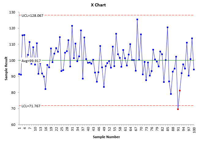
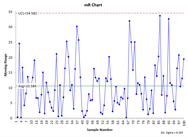
What do these two charts tell you?  The second chart, the moving range (mR) chart, is in statistical control. There are no points beyond the control limits or any patterns.  Since it is in control, you can estimate the standard deviation (s). 

σ =  R̅/1.128 = 10.584/1.128 = 9.383

The X chart does have two out of control points, one due to points beyond the control limits and the other due to the Zone A test.  Does this mean that the process is out of statistical control?  It is pretty consistent and predictable.  Only two out of control points out of 100.  I would say this process is consistent and predictable.  Of course, you should find out what caused those two points to be out of control.

What does the Rameriz-Runger statistic say about this control chart?  The global standard deviation (s) is 9.704. 

Rameriz-Runger Statistic = (s/s)² = (9.704/9.383)² = 1.07

This value is close to 1, so you would assume that the process is in statistical control.  Now to calculate the p-value.  There are 100 data points so the degrees of freedom associated with s is 100 -1 = 99. The degrees of freedom associated with s is 0.62(n-1) = 61.38 which rounds down to 61. The p-value is:

p-value = FDIST(1.07, 99, 61) = 0.392

With this value of p, it is probably reasonable to believe that the process is in statistical control.  It is considerably higher than the 0.05 which is used with many statistical tests.  And the process does appear to be fairly consistent and predictable. 

Out of Statistical Control Example

Consider the data in Table 2.  We will use this data to see what happens with the Rameriz-Runger statistic with a process that is out of statistical control

Table 2: Out of Statistical Control Example

The individuals (X-mR) control charts are shown in the figure below.

Figure 2: Table 2 X-mR Control Charts

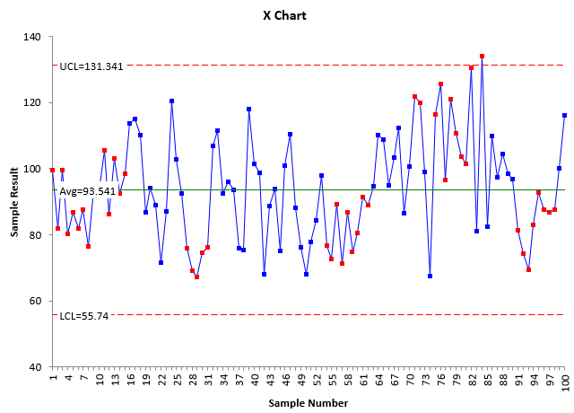
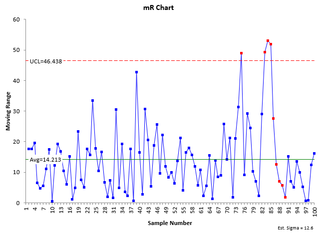
Both charts in Figure 2 have out of control points.  Since the mR chart is out of statistical control, we really can’t estimate the variation (s), but we will do it anyway.

σ =  R̅/1.128 = 14.213/1.128 = 12.600

The X chart has multiple out of control points.  The global standard deviation is 15.583. Then:

Rameriz-Runger Statistic = (s/s)² = (15.583/12.600)² = 1.53

The p-value is:

p-value = FDIST(1.53, 99, 61) = 0.037

Since this p-value is “small”, the probability of the process being in statistical control is low.  You would conclude that the process is out of statistical control, which is confirmed by the actual control chart.

The Simulations

We have examined two examples trying to see if the Rameriz-Runger statistic can be used to determine if a process is in statistical control.  It appears promising.  Enter variation.  As we continue to take data, we won’t get the same result each time – even if the process is in statistical control.

To examine the Rameriz-Runger statistic in more detail, three simulations were run.  The first simulation is a process that is in statistical control.  The second simulation is for a process that is widely out of control.  The third simulation is a mixture of two processes with their averages differing by one standard deviation. The standard deviation  in the simulations was the same.

Simulation 1

10,000 data points were randomly generated for a normal distribution with an average of 100 and a standard deviation of 10.  These 10,000 data points represent the entire universe – all the possible results.  100 data points were selected at random from these 10,000 points,  and a control chart was created for those 100 data points.  The control chart should be in statistical control.  The following were calculated for the control chart:

• • The global standard deviation
  • The average moving range
  • The estimated sigma (R̅ /1.128)
  • The Rameriz-Runger statistic
  • The p-value

This was repeated 1,000 times.  Figure 3 is an example of one of the X charts from the simulation.  We will not worry about the moving range chart here.

Figure 3: X Chart for Simulation 1

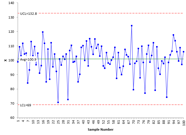
It is in statistical control.  This particular chart has a Rameriz-Runger statistic of 0.917 and a p-value of 0.654.  This would imply that the process is in statistical control.  But what about the other 999 control charts from the simulation.  Table 3 lists the minimum, average, and maximum for each of the calculated variables:

Table 3: Simulation 1 Results

Note the wide range of results.  The value of s varies from 7.61 to 12.33.  All the variables have variation. Focusing on the p-value, it varies from 0.03 to 0.95.  Figure 4 below shows the Rameriz-Runger statistic versus the p-value.

Figure 4: Rameriz-Runger Statistic vs p-Value for Simulation 1

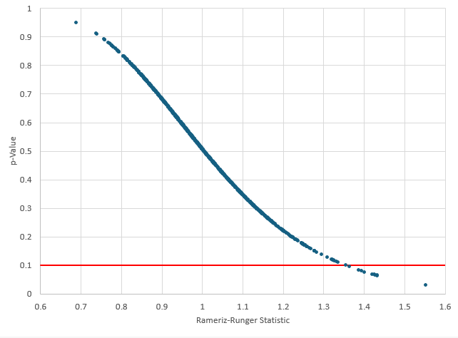
There is a large range of p-values with the simulation.  Suppose you select a p-value of 0.10 as the cutoff.  If the p-value is greater than 0.10, you conclude that the process is in statistical control.  If it is less than 0.10, you conclude that the process is not in statistical control.  The red line in Figure 4 represents p = 0.10.  Of the 1000 p-values in this simulation (which assumed an in control process), 11 are less than 0.10.  That means you would have made the wrong choice 11 times out of 1,000.  Not too bad.  So, for an in control process, the Rameriz-Runger statistic seems to work pretty well. 

Simulation 2

This simulation involves a process that is out of statistical control.  It bounces around.  The 10,000 points were generated using a normal distribution by randomly selecting 2000 points with these averages: 100, 150, 80, 70 and 125. The standard deviation for each was 10.  Figure 5 is an example of an X control chart with this simulation.

Figure 5: X Chart for Simulation 2

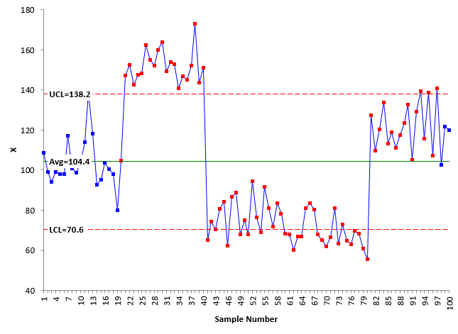
This chart is widely out of control.  Table 4 summarizes the results.

Table 4: Simulation 2 Results

There is a wide range of results again in the data.  But look at the p-values.  They are very, very small.  You would conclude for all these p-values that the process is out of control.  This implies that the Rameriz-Runger statistic will work with control charts that are widely out of control, with large shifts moving up and down.

Simulation 3

This simulation attempts to find a midpoint between simulation 1 and simulation 2.  For this simulation, 2500 points were randomly generated using a normal distribution for process averages of 100, 110, 100, and 110.  Again the standard deviation used in generating the random numbers was 10.  Figure 6 is an example of a control chart from this simulation.

Figure 6: X Chart for Simulation 3

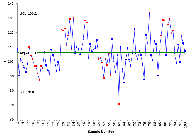
This chart shows some out of control points, not as many as Simulation 2.    The results are summarized in Table 5.

Table 5: Simulation 3 Results

Again, there is a lot of variation in the simulation results.  Figure 7 shows how the p-value varies with the Rameriz-Runger statistic.

Figure 7: Rameriz-Runger Statistic vs p-Value for Simulation 3

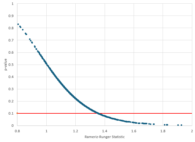
Suppose you use the cutoff point for the p-value to be 0.10.  This is the red line in Figure 7.   205 times with this simulation, the p-value was less than 0.10.  So, you would conclude that the process was out of statistical control.  But 795 times the p-value was greater than 0.10, implying that the process is in statistical control.  This is a problem. The process is definitely not in statistical control, but the Rameriz-Runger statistic says it is about 80% of the time.

Summary

Can the Rameriz-Runger statistic be used as process stability index?  That one number that will tell us if the process is in statistical control or not. Unfortunately, the answer is no.  It appears to be able to identify wildly out of control processes, like shown in Simulation 2.  Simulation 1 shows that the statistic can confirm that a process is in statistical control the vast majority of times. However, for processes that are borderline out of control (or a little more than that as shown in simulation 2), the statistic indicates that the process is in statistical control when it is not.  All the statistic can really do is to tell if you the process is widely out control. It is not of much use beyond that for predicting statistical control.

What do you do?  Just what Dr. Wheeler most likely would tell you to do.  Make the control chart and check the stability before you start any other statistical tests.