Equivalence Testing

November 2024

Equivalence Testing  is one of the new techniques in the just release SPC for Excel version 7.  To view what is new in version 7, please select this link. To see all the statistical tools in SPC for Excel, please select this link.

You are looking to replace an older measurement system with a new one. You want to know if the new measurement system is the “same” or “equivalent” to the old one. Note that you don’t want to know if they are different.  You want to know if they are the same. In this case, the “same” means that the difference between the two measurement systems are within a predefined margin of error. If the difference is within that margin of error, then the observed differences are not meaningful in the practical sense.

There are several equivalence testing methods including one sample, two sample and paired samples equivalence testing. This publication introduces equivalence testing, in particular the two sample equivalence test

In this publication:

• Introduction
• Example Data
• Calculations for Two Sample Equivalence Test
• Conclusions from the Two Sample Equivalence Test
• Other Alternate Hypotheses
• Comparison to the Two Sample t Test
• Other Equivalence Tests
• Summary
• Quick Links

Feel free to leave a comment at the end of this publication.  You canb download a pdf copy of this publication at this link.

Introduction

Suppose you work in a heat treating facility. You routinely measure the hardness of steel samples using a Rockwell hardness tester. The tester you are using has been around for a number of years and you are having more and more problems with it. You ordered a new hardness tester that has arrived and been set up. You want to know if the new hardness tester gives the same results as the old hardness tester.

To use equivalence testing, you must decide on the range within which the differences in the two testers are trivial or not of practical significance. This is your margin of error or equivalence interval. Suppose you decide that it is practically insignificant if the difference in the means of the two testers is within ± 0.5 Rockwell hardness.

You are performing a hypothesis test with equivalence testing. The null hypothesis (H₀) and the alternate hypothesis (H₁) for this example are given below.

H₀: The difference in the means of the two testers is outside the equivalence interval

H₁: The difference between the means is inside the equivalence interval and the means are equivalent

To perform equivalence testing, you collect your samples and run the samples in the old tester and the new tester. You then perform the calculations as shown below. Two key calculations are key to interpreting the results.

One is a confidence interval that is calculated. This interval is a range that contains the difference between the two means. If the confidence interval fits entirely within the equivalence interval (± 0.5 in this example), you conclude that the two testers are the same. If the confidence interval does not fit entirely within the equivalence limits, you conclude that the two tests are considered different.

The other key calculation involves the p-value. To perform this calculation, you have to decide on the value of alpha. Alpha (a) is called the significance level. Typical values of alpha are 0.05 and 0.10. The significance level gives the risk of accepting the null hypothesis when you should not. A value of 0.05 means that risk is 5%. This is also related to the confidence interval. If alpha = 0.05, the confidence interval is a 95% confidence interval.

A t-value is calculated. The p-value represents the probability of getting that t statistic if the null hypothesis is true. If the value of p is small, then we conclude that the probability of getting that t-value, if the null hypothesis is true, is small and reject the null hypothesis. If the p-value is large, we conclude that the probability of getting that t-value if the null hypothesis is true is large and we accept the null hypothesis.

We examine how this works with the example below.

Example Data

To test this, you take 50 samples at random from your process and test 25 of them in the old hardness tester and test 25 of them in the new hardness tester. The results are given in Table 1.

Table 1: Old and New Hardness Testers Results

The data will be used to show how the calculations for the two sample equivalence test are done.

Calculations for Two Sample Equivalence Test

The SPC for Excel software was used to analyze the data. How those results were calculated is given below. The first step is to calculate the following sample statistics.

Sample Statistics

The statistics calculated include the sample size, the average (the mean), the standard deviation, and the standard error the mean (SE Mean). The SE Mean estimates the differences between means you would obtain if you repeated taking samples from the same population. It is given by the square root of the standard deviation squared divided by the sample size:

where s = the standard deviation and n = sample size.

The next step is to calculate the difference statistics:

The difference is simply the difference in the old tester average and the new tester average. SE is the standard error of the difference and is given by:

Subscript 1 refers to the test sample, while subscript 2 refers to the reference sample (old and new, respectively). The standard error of the difference estimates the variation in the differences between the two means if repeated samples are taken from the same populations and the difference in the averages calculated.

The next step is to compare the equivalence limits (or interval) to the calculated confidence limit for the difference in the averages.

The equivalence limits are what you selected, in this example +/- 0.5.

To calculate the confidence interval, we need to select a value of alpha. We will use 0.05. The confidence interval gives a range of values for the difference between the two averages. The lower limit is the lowest difference you would expect while the upper limit is the largest difference you would expect.

You can perform two-sided or one-sided confidence intervals. We will do a two-sided confidence interval here. The equations for calculating the two-sided confidence intervals are given below.

Lower Confidence Limit = minimum of (C, D_L)

Upper Confidence Limit = maximum of (C, D_u)

where

C = (LEL+UEL)/2

D_L = Difference in averages – t(SE)

D_u = Difference in averages + t(SE)

where LEL is the lower equivalence limit (-0.5 in this example), UEL is the upper equivalence limit (0.5 in this example) and t is the t value from the t distribution. The t value depends on 1 – alpha and the degrees of freedom.

The degrees of freedom (df) is given by the following:

If you enter the values in the above equation and round down, you will get df = 47. You can use the Excel function T.INV to find the value of t:

t = T.INV(1– alpha, df) = T.INV(0.95, 47) = 1.678

Now we can calculate the confidence interval.

C = (LEL+UEL)/2 = (-0.5 + 0.5)/2 = 0

D_L = Difference in averages – t(SE) = 0.38 – 1.678(0.220) = 0.011

D_u = Difference in averages + t(SE) =0.38 + 1.678(0.220) = 0.749

and

Lower Confidence Limit = minimum of (C, D_L) = minimum of (0, 0.011) = 0

Upper Confidence Limit = maximum of (C, D_u) = maximum of (0, 0.749) = 0.749

So, the confidence interval is 0 to 0.749.

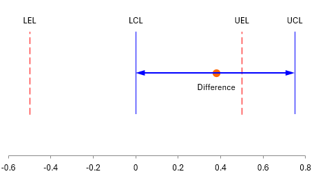
This gives you the first indication if the two testers are the “same” when you compare the confidence interval to the equivalence interval. If the confidence interval fits within the equivalence interval, you conclude that the two tests are the same. Figure 1 compares the two.

Figure 1: Confidence Interval Compared to Equivalence Interval

The figure plots the difference in the averages. The blue line shows the confidence interval. You can see it does not fit within the equivalence interval. So, it does not look like the two testers are the same.

The next step is to test the null hypothesis. The output from the SPC for Excel software is shown below.

Hypothesis

H0: Difference <= LEL or Difference >= UEL

H1: LEL < Difference < UEL

As shown in the results, there are two null hypothesis tests. One hypothesis is that the difference in the two averages is less than LEL; the other is that the difference is greater than the UEL.

The equations for the t-values are given below, with subscript 1 for the hypothesis difference ≤ LEL and subscript 2 for the hypothesis difference ≥ UEL.

t₁ = (Difference – LEL)/SE = (0.38 – -0.5)/0.22 = 3.997

t₂ = (Difference – UEL)/SE = (0.38 – 0.5)/0.22 = -0.5451

Now, we calculate the p-value for each t-value. Remember the p-value is the probability of getting the t-value if the null hypothesis is true. We can use two of Excel’s t distribution functions to determine the p-value as shown below:

p₁ = T.DIST.RT(t₁, df) = T.DIST.RT(3.997, 47) = 0.0001

p₂ = T.DIST(t₁, df, TRUE) = T.DIST(3.997, 47, TRUE) = 0.2941

Both these p-values must be less than the value of alpha we selected (0.05). One of them is not, so we cannot assume that the two testers are the same.

Conclusions from the Two Sample Equivalence Test

Based on the analysis above, we conclude that the old tester and the new tester are not equivalent. The two points that allow us to reach this conclusion are the following:

1. The confidence interval does not fit entirely within the equivalence interval (see Figure 1).
2. The maximum p-value for the null hypothesis is greater than the value of alpha selected (0.05 in this example).

Other Alternate Hypotheses

The example above used the following alternate hypothesis:

H₁: LEL < Difference in the averages < UEL

You can also use any of the following alternative hypotheses depending on what you are trying to find out:

H₁: Test Average > Reference Average

H₁: Test Average < Reference Average

H₁: Difference > LEL

H₁: Difference < UEL

Comparison to the Two Sample t Test

The two sample equivalence test appears to be very similar to the two sample t test. The two sample t test is used to determine if there is a statistically significant difference between the averages of two populations. The null and alternate hypotheses for the two sample t test are:

H₀: m₁ = m₂

H1: m₁ ≠ m₂

where  m represents the average. If the p-value for the two sample t test is less than alpha, you conclude that the two averages are different.

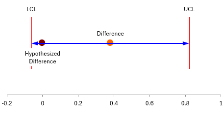
The data in Table 1 was analyzed using the t test for the difference in two means with the SPC for Excel software. Figure 2 plots difference in the two averages with the confidence interval.

Figure 2: t Test for the Difference in Means

You can see from Figure 2, that the hypothesized difference of zero lies with the confidence interval, so we conclude that the difference in the old tester and new tester averages can be zero – that the testers are the same. The p-value in this example is 0.091, which is greater than 0.05. So, more evidence that the two tests have the same average.

With the equivalence testing, we defined a range of values for the difference in the averages that was not practically important. It didn’t matter to us if the difference ranged from -0.5 to 0.5. The difference of 0.38 falls in that range, so from an equivalence point of view, it is not significant.

If you have a range that is not significantly important to you, you should consider using the equivalence test instead of the standard t test.

Other Equivalence Tests

There are other equivalence tests than the two sample test. Two of these are:

1. One-Sample Equivalence Test: this test is used to determine if the average of a population is close enough to a target value.
2. Paired Samples Equivalence Test: this test is used to determine if the mean of a test population is close enough to the mean of a reference population using paired samples (each sample tested in each population).

In these tests, the “close enough” refers to the equivalence interval you select.

Summary

This publication introduced equivalence tests with a focus on the two sample equivalence test. In equivalence testing, the user selects a range of values that the user considers are not important in the practical terms. This is called the equivalence interval. In the two sample case, if the confidence interval falls within the equivalence interval, the two populations are considered the same. The analysis in this publication was done using the SPC for Excel software.