Comparing Two Proportions

May 2024

Sometimes we want to compare the proportions in two populations with binary outcomes (e.g., success or failure) to determine if the proportions are the same or if the proportions are different.  For example, we might want to know if the proportion of males who vote in an election is the same or different than the proportion of females who vote in that election.   You might want to compare two drugs to see if the impact of treating a disease is the same or not. 

There is a statistical test – comparing two proportions – that helps us do this.  To use this test, data is collected from each of the two populations (for example, men and women).   The data collected is the sample size, the number of successes and the number of failures for each population.  These data can then be used to determine if there is a statistically significant difference in the results from the two populations.  This publication describes how to do this.

In this publication:

• Example 1
• The Hypothesis
• The Math
• Interpretation of the Math
• Pooled Estimate of p
• Example 2
• Other Considerations
• Summary
• Quick Links

Please feel free to leave a comment at the end of the article.  You can also download a pdf copy of this publication at this link.

Example 1

We will introduce the calculations using an example involving high school students and smoking.  One city, City A, has implemented a new smoking cessation program aimed at high school students.  Another city, City B, has not implemented the program.  We want to know if there is a statistically significant difference  in the two cities in the proportion of high school students who have smoked during the last six months.

In City A, 210 students from a sample of 950 high school students had smoked cigarettes in the last six months.  In City B, 255 students from a sample of 1300 high school students have smoked cigarettes in the last six months.  We want to know if there is a statistically significant difference between the two cities.

This situation represents where the two proportion test can be used.  You have a population of high school students in population 1 (City A).  And you have a population of high school students in population 2 (City B).  It doesn’t matter which one is population 1 or population 2.  For each population there is a “true” value for the proportion of high school students who have  not smoked cigarettes in the last six months.  We will denote those “true” proportions as p₁ and p₂, respectively for population 1 and population 2.

You usually can’t ask each student in each city about smoking cigarettes to determine the “true” proportions.  Instead, you take a sample from each city. In this example, we took a sample of 950 from City A and a sample of 1300 from City B.  For each sample, certain statistics are calculated as shown in the table below.

Table 1: Two Proportions Calculations

Note that q̂₁  = 1 – p̂₁ for City A.  The same holds for City B.

The proportion who has not smoked in the last 6 months is 0.779 for City A and 0.804 for City B.  It is not surprising that there is a difference between the two numbers.  After all, we  are taking a sample and there is variation present.  The question is whether or not the two numbers are significantly different statistically.  The two proportion test will answer that question for us.

The two proportion test described below is the large sample case.  The large case is used if the following is true:

The Hypothesis

We will use the two-tailed test in this example.  The null hypothesis (H₀) for the two-tailed test is that the two population proportions are the same:

H₀:  p₁ – p₂ = 0

The alternate hypothesis (H₁) is that the two population parameters are not equal:

H₁:  p₁ – p₂ ≠ 0

The Math

For large samples, you can assume that the samples from the populations are normally distributed.  This allows you to calculate the z statistic to help determine if the difference between the two proportions is zero or not.  The z statistic measures how many standard deviations a value is from the hypothesized difference of 0.

There are two ways to tell if there is a significant difference between the two proportions.  One looks at the 95% confidence interval around p₁ – p₂.  If this interval contains 0, we will conclude that there is no evidence that the proportions are different (e.g., accept H₀).  If the 95% confidence limit does not contain zero, we will conclude that there is evidence that the proportions are not equal. 

The second method looks at the calculated p-value.  The p-value can be looked at as the probability of getting the calculated z statistic if the H₀ is true.  If that probability is small, then we conclude that there is evidence that the proportions are not equal.  “Small” is determined by the value of alpha you select.  Usually, alpha is 0.05.   The confidence limits are set at 1 – alpha, or 1 – .05 = 95% when alpha = 0.05.

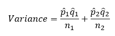
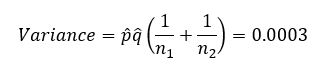
We will start by calculating the z statistic.  We need a measure of variation to do that.  The variance is estimated as the following:

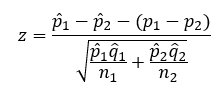
You can then calculate the z statistic as follows:

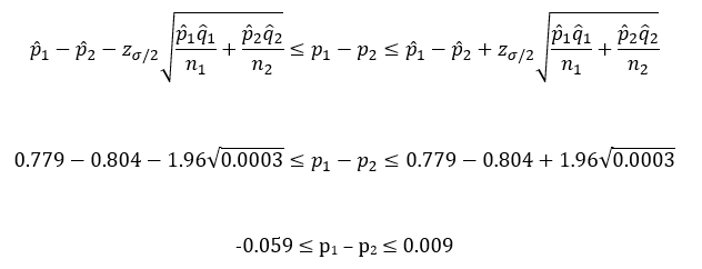
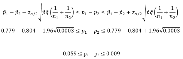
The 100(1- s)% two-sided confidence interval for p₁ – p₂ is then:

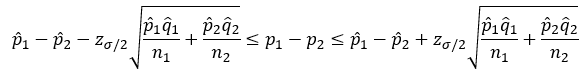
The z_s/2 in the equation above is not the z statistic.  The z term, z_s/2, is referring to the z critical value from a z table that corresponds to s/2.   Since this is a two-sided test, you divide alpha by two.  In this example, s/2 = 0.025 since we chose alpha = 0.05.  The value of  z_s/2 for alpha = 0.05 is 1.96.

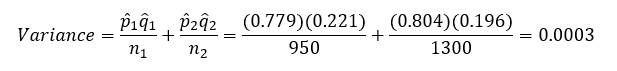
Let’s begin to put some numbers in to do the calculations, starting with the variance:

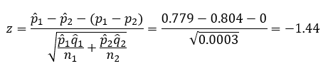
Now, calculate the z value:

Finally, calculate the 95% confidence interval:

Interpretation of the Math

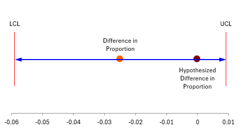
We have done the calculations; now to interpret the results.  As stated before, there are two ways we will determine if the two proportions are the same or different.  One of those is the 95% confidence interval.  The lower confidence limit for this example is -0.059; the upper confidence interval is 0.009.  All values between the confidence limits are possible values for the difference in the two proportions.  Since the confidence interval contains 0, we conclude that is possible for the two proportions to be equal and accept the null hypothesis.

You can also see this easily in the plot below.  The hypothesized difference is within the confidence limits.  There is no evidence that the two cities have a different proportion of high school students who have not smoked in the last six months. 

The second method of determining if there is a difference in the two proportions is through the z value.  The z statistic for this example is -1.44.   The question to answer is what is the probability of getting this z statistic if the null hypothesis is true – that there is no difference in the two proportions.  To find this probability, you can use the following function in Excel (for the two-sided confidence interval):

p-value =2*(1-NORM.S.DIST(ABS(z),TRUE)

This gives a p-value of 0.15.  This means that there is about a 15% probability of getting this z value or one more extreme if the null hypothesis is true.  We chose alpha = 0.05.  Since the p-value is greater than alpha, we conclude that there is no evidence that the two proportions are not equal.  The null hypothesis is accepted.

Pooled Estimate of p

It should be noted that sometimes the two p values are pooled to get a “better” estimate of the true proportion.  If H₀ is true, then both p₁ and p₂ are estimating the same true population, p.  The pooled estimate of p is given by:

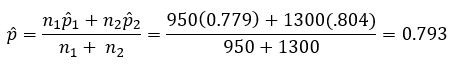
The  pooled estimate for this example is 0.793.  The z statistic equation is slightly different and is then given by:

The variance of the pooled estimate is given by:

The 95% confidence limits are given by:

The z statistic and the  95% confidence limits are essentially the same as before.  This is because the two proportions are essentially the same.  You will see differences when there are larger differences in the two proportions.

Example 2

The following example is from Penn State’s online statistical course. 

“Time magazine reported the result of a telephone poll of 800 adult Americans. The question posed of the Americans who were surveyed was: “Should the federal tax on cigarettes be raised to pay for health care reform?” The results of the survey were:”

These data were analyzed using the SPC for Excel software.  The output is shown below.

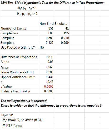
The output shows the results of the calculations covered above.  The p-value is very small (essentially zero) and the confidence interval does not include 0, so there is evidence that the difference between smokers and non-smokers is not 0 and the null hypothesis is rejected. The chart below (part of the output from the SPC for Excel software) confirms this.

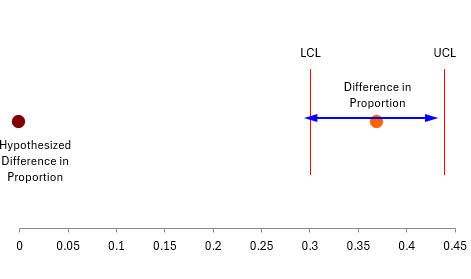
The hypothesized difference in proportions is outside the confidence limits.

Other Considerations

The procedure outlined in this publication is the large sample case.  There is also a procedure for the small sample case.  This procedure will not be covered here but it is done in the SPC for Excel software as well.  It is called the Fisher’s Exact Test.  The p-value for that test is given in the output shown above.  You can also perform one-sided confidence intervals and not just the two-sided process shown here.

Summary

This publication showed the mathematics behind comparing two proportions to determine if they are equal or not.  The two things to help decide that are the confidence interval and the probability of getting the calculated z statistic.   If the confidence interval does not contain 0, there is evidence that the two proportions are not the same.  If the p-value is small, there is also evidence that the two proportions are not the same.