Comparing Four Normality Tests

May 2025

Suppose you have a set of data, and you want to apply some statistical tests to the data. You read up on some of the tests, and you discover that the test assumes the data are normally distributed.

How do you find out if your data are normally distributed? You can make a histogram and see if it looks like that familiar bell-shaped curve. If it does, you can assume that the data are normally distributed. You can also construct a normal probability plot to see if the data falls along a straight line for the most part. If it does, you can assume that the data are normally distributed.

But some of us like numbers. Is there a statistic that will tell us if the data are normally distributed? Yes, several, when used in combination with a p-value.

This publication looks at four different normality tests: the Anderson-Darling (AD) test, the Kolmogorov-Smirnov (KS) test, the Lilliefors test, and the Shapiro-Wilk (SW) test. An explanation of how each test works is given, along with the steps in using each test.

In this publication:

• The Hypotheses
• Example Data
• Anderson-Darling (AD) Test
• Kolmogorov-Smirnov (KS) Test
• Lilliefors Test
• Shapiro-Wilk (SW) Test
• Which is Best?
• Summary
• Quick Links

All four normality tests are included in the SPC for Excel software.

Please feel free to leave a comment at the end of the publication.  You can download a pdf copy of the publication at this link.

The Hypotheses

The two hypotheses for the four normality tests are given below:

H₀: The data follows the normal distribution

H₁: The data do not follow the normal distribution

Our approach for each test will be to calculate a statistic for the example data and then determine the p-value for that statistic to help us determine if the data are normally distributed or not. Remember the p (“probability”) value is the probability of getting a result that is more extreme if the null hypothesis is true. If the p-value is small (e.g., <0.05), you conclude that the data do not follow the normal distribution. If the p-value is large (e.g., > 0.05), you conclude that the data are normally distributed.

Remember that you choose the significance level even though many people just use 0.05 the vast majority of the time. The significance level is often called alpha (a). We will use alpha = 0.05 in this publication.

Example Data

Suppose we have a dataset of 50 samples. We want to know if this data is normally distributed. The data are shown in Table 1.

Table 1: Example Data

One way of seeing if you have a normal distribution is to construct a histogram. The histogram for these 50 samples is shown in Figure 1.

Figure 1: Example Data Histogram

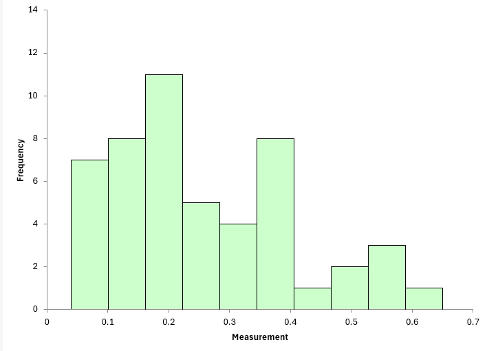
Does the data in the histogram look like a normal distribution? With just 50 data points, it is sometimes hard to know for sure. It looks like it might be a stretch to call this a normal distribution.

So, we can make a normal probability plot and see if the points fall along a straight line. Figure 2 shows the normal probability plot for the data.

Figure 2: Normal Probability Plot

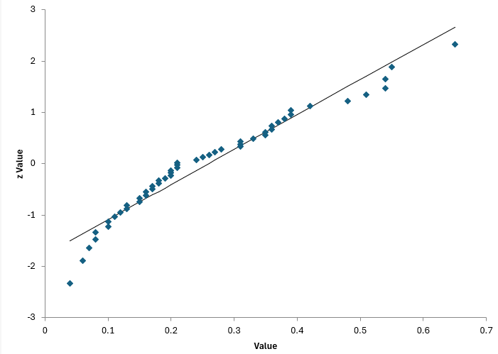
Do the points tend to lie along the straight line? Some do, some don’t. It is probably questionable if this comes from a normal distribution.

But to confirm it further, we can use one of the four tests above. In fact, we will use all four to see if there are differences, starting with the Anderson-Darling statistic.

Anderson-Darling (AD) Test

The Anderson-Darling test was developed in 1952 by Theodore Anderson and Donald Darling. This test checks whether a dataset comes from a normal distribution (it works with other distributions as well) by comparing the actual distribution of the data to what you would expect if the data were normally distributed.

The test involves calculating the AD statistic and then determining the p-value for that AD value.

The steps in the calculation of AD are given below.

• Sort the n samples from smallest to largest
• Calculate the average and the standard deviation (s) of the data
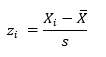
• Standardized the data using:

• Calculate the cumulative distribution function (CDF) for the normal distribution for each z value: F(z_i). This calculates how far off the data are from the expected values of a normal distribution (using the mean and standard deviation of the sample data).
• Calculate the AD statistic as shown below. The value of AD summarizes how different the sample data is from a true normal distribution. The higher the value, the less likely the data is to be from a normal distribution.

The equation above for AD puts more weight on the differences between the sample data and a true normal distribution in the tails. It does this through these two terms in the equation: lnF(X_i) and ln(1-F(X_n-i+1)) . These terms become large when they are close to 0 and 1, i.e., in the tails. So, the AD test is sensitive to differences from a normal distribution in the tails.

For the data in Table 1, the calculated value of AD is 0.2993.

The value of AD needs to be adjusted for small sample sizes. The adjusted AD value is given by:

For the data in Table 1, AD* = 0.8791.

Does the value of AD* imply the data are normally distributed? You don’t know using the value of AD* by itself. This is determined by the p-value.

The calculation of the p-value for the AD test is not straightforward. The reference most people use is R.B. D’Augostino and M.A. Stephens, Eds., 1986, Goodness-of-Fit Techniques, Marcel Dekker.

There are different equations depending on the value of AD*. These are given by:

• If AD*=>0.6, then p = exp(1.2937 – 5.709(AD*)+ 0.0186(AD*)²)
• If 0.34 < AD* < .6, then p = exp(0.9177 – 4.279(AD*) – 1.38(AD*)²)
• If 0.2 < AD* < 0.34, then p = 1 – exp(-8.318 + 42.796(AD*)- 59.938(AD*)²)
• If AD* <= 0.2, then p = 1 – exp(-13.436 + 101.14(AD*)- 223.73(AD*)²)

The value of AD* for our example falls in the range of the first bullet above. Substituting in the value of AD* into the equation gives the p-value = 0.0245. Since this probability is low (2.45%), we assume that the null hypothesis is false, and the data are not normally distributed.

Kolmogorov-Smirnov (KS) Test

Two mathematicians, Andrey Kolmogorov and Nikolai Smirnov, developed this test in the 1930s. This test is a non-parametric test used to determine if a sample comes from a normal distribution. It can be used with other distributions also. The KS test compares the empirical distribution function (EDF) of the sample with the cumulative distribution function (CDF) of the normal distribution.

The steps in the calculation of KS are given below.

• Sort the n samples from smallest to largest.
• Calculate the average and the standard deviation (s) of the data
• Standardized the data using:

• Calculate the empirical CDF:

• Calculate the theoretical normal CDF: F(z_i) ; you can use the Excel function NORM.S.DIST for this calculation.
• Calculate D+ and D-:

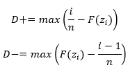
• Calculate D, which is the maximum of D+ and D-.

Note that D+ is the maximum positive deviation between the empirical CDF, F_n(z_i), and the theoretical CDF, F(z_i). D- is the maximum negative deviation. D is the larger D+ and D-.

The value of KS for the data in Table 1 is D = 0.1515. You can’t simply compare the normality statistics to find anything out. You have to go to the p-values each time. There are tables of critical values for D to compare the calculated D value to. You can also use the equations below to determine the p-value.

The p-value from the above equation converges rapidly usually. The p-value for the example data in Table 1 is 0.1844. Note that it is larger than 0.05, which would imply that the data are normally distributed.

This conflicts with the Anderson-Darling results. What is going on? There is a problem with using the p-values calculated as shown above for the KS test. It is conservative when used with the average and standard deviation calculated from the sample. The KS test is really designed to be used with known average and known standard deviation from the distribution population – the “true” values – which we seldom know. This leads to the KS test failing to reject that the data comes from a normal distribution when it should reject it.

You should use a modified KS test with the Lilliefors p-value.

Lilliefors Test

The Lilliefors test was developed in 1967 by Hubert W. Lilliefors, an American statistician. Lilliefors adjusted the critical values for D to account for using the sample averages and standard deviations.

The Lilliefors test accounts for the fact that the mean and standard deviation are estimated from the data, which affects the distribution of the D statistic.  The calculation of the D statistic is the same as for the KS test.

The difference is in determining the p-value associated with that D value. The easiest way to get this p-value is from a table of Lilliefors critical D values. You look up the critical D value in the table based on n = sample size and alpha = significance level and then decide based on the following:

D < D_critical: Assume that the data does come from a normal distribution

D > D_critical: Assume that the data does not come from a normal distribution

You can also use interpolation to find the p-value. Doing this gives a p-value < 0.01 for the data in Table 1. This definitely says that the data are not normally distributed.

You can download a table of the critical D values at this link.

Shapiro-Wilk (SW) Test

The Shapiro-Wilk test was developed in 1965 by Samuel Shapiro and Martin Wilk to test for normality. It is only used to determine if the data is normally distributed or not. It is not used with other distributions. The steps in performing the SW test are given below.

• Sort the n samples from smallest to largest.
• Determine the values of mi using:

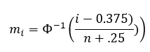
            where Φ ^-1  is the inverse of the standard normal cumulative distribution (NORM.S.INV in Excel) and i is the i^th number in sorted data.

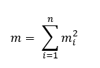
• Calculate m.

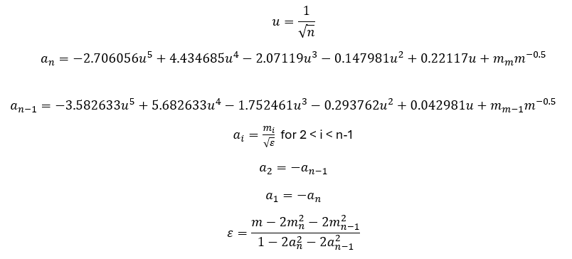
• Calculate the a_i coefficients.

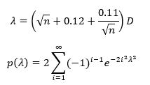
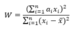
• Calculate the W test statistic:

• Determine the p-value.

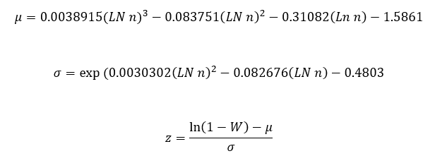
            The p-value is 1 – NORMSDIST(z).

For the data in Table 1, W = 0.9438. W is a measure of how close the data is to a normal distribution.  The p-value associated with that value of W is 0.0191. This is less than 0.05, so we conclude that the data does not come from a normal distribution.

Which is Best?

The results for the data in Table 1 are shown in Table 2 below.

Table 2: Normality Results

The Kolmogorov-Smirnov test incorrectly assumes that the data are normally distributed. The other three tests correctly point out that the data are not normally distributed.

Of course, one data set doesn’t tell us for sure which tests are better. From the literature, it appears that the following is true for detecting normality.

The Shapiro-Wilk test has the best power for detecting distributions that are not normal. It is good for sample sizes less than 5000.

The Anderson-Darling test is next. It is very powerful especially in the tails of the distribution.

Next is the Lilliefors test. It is more powerful than the KS test since it takes into account calculating the average and standard deviation from the sample.

And last is the Kolmogorov-Smirnov test. It is only good if you know the true average and standard deviation of the population.

Summary

This publication reviewed four different normality tests.  The steps in using each test were covered. A statistic for each test is calculated with a p-value calculated to determine if the data are normal or not. For normality studies, the Shapiro-Wilk and the Anderson-Darling test are the best.