Binary Logistic Regression Help
Home » SPC for Excel Help » Cause and Effect Help » Binary Logistic Regression Help
Binary logistic regression is used to determine the relationship between predictors (continues and/or categorical) a response variable that only has two possible outcomes. The outcomes can be yes/no, pass/fail or any binary response. For example, you may do a study to determine who will buy a product or not buy it or who will vote or not vote in election. The binary logistic regression methodology will identify which predictors have a statistically significant impact on the response variable.
The example below shows how to use binary logistic regression in SPC for Excel. This page contains the following:

Example
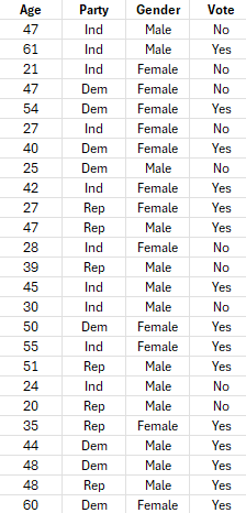
A student wants to determine the impact that age, party affiliation, and sex has on whether a person votes or not. The student collects data on 25 randomly selected people. Please see this link for how SPC for Excel handles categorical predictors if you have them.
Data Entry
Enter the data into a spreadsheet as shown below. The data can be downloaded here. The data must be in columns with the variable names in the first cell of the column.
Running the Binary Logistic Regression
- 1. Select data on the spreadsheet including the headings. You can use “Select Cells” in the “Utilities” panel of the SPC for Excel ribbon to quickly select the cells.
- 2. Select “Regression” from the “Cause and Effect” panel on the SPC for Excel ribbon.
- 3. Select “Binary Logistic Regression."
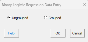
- 4. The binary logistic regression data entry screen is shown below. Select whether you data is ungrouped (one data point per event, as in this example) or grouped (summary data). The default is grouped.
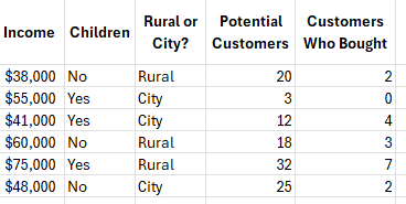
- 5. An example of grouped data is shown below. In this grouped example, the number of customer who bought a product is the event. The number of trials are the potential customers. The predictors are income, whether they have children, and whether they are rural or live in the city.
- 5. Selecting OK, shows the form binary logistic regression input for ungrouped data.
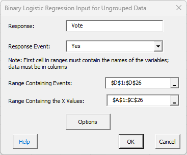
- Response: this is the name of the response; the default value is the first cell in the range containing the events if it is non-numeric.
- Response Event: select the response that will count as an event; two will be listed in the dropdown box.
- Range Containing Events: the worksheet range containing the events (the response variable)
- Range containing X values: the worksheet range containing the X values
- Options: selecting options displays the input form below.
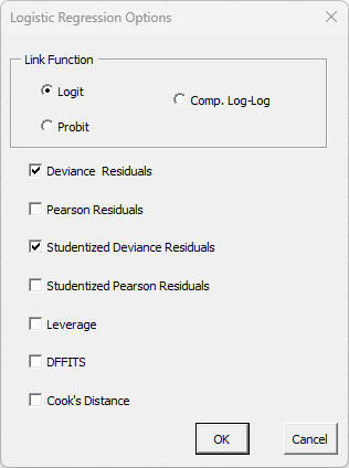
- Link Function: select either Logit (the default), Probit, or Comp. Log-Log.
- The default residuals are checked. You can change those options.
- Select OK or cancel to return to last input form. Then select OK to generate the binary logistic regression analysis or select Cancel to exit the SPC for Excel program.
Binary Regression Regression Output
There are four new worksheets added during the analysis:
- Data (1)
- Summary (1)
- Residuals (1)
- Regression Charts (1)
The number in parentheses is the number of regressions in the workbook. This allows you to keep track of the worksheets that go together when you remove observations, remove variables, or transform the Y variable and rerun the regression. The ranges containing the results on the first three sheets listed are protected. This is necessary for the program to find the information needed to rerun the regression. The four worksheets are described below.
Data
This worksheet contains the data used in the regression analysis.
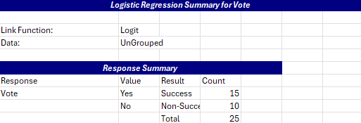
Summary
Most of the output for the binary logistic regression is shown on the Summary worksheet. The top part of the Summary sheet shows the link function and the response summary. This includes the number of successes and non-successes.
The deviance table is shown next.
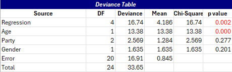
It is used to define which variables have a significant impact on the response variable. If the p-value for the source is less than 0.05, the variable has a significant impact on the response. If the p-value for the source is greater than 0.05, you might consider removing it from the model, as shown below. In this example, Age is statistically significant. If the p-value is less than 0.05, it is shown in red.
Age is a continuous predictor. If it is statistically significant, it means that the coefficient for temperature is different than 0. Party is a categorical predictor. If a categorical predictor is statistically significant, then it means that the levels (like Rep and Dem) don’t have the same average.
The next output on the Summary worksheet is the predictor’s table.
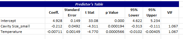
This contains the coefficients, standard error, t statistic, p value, the 95 % confidence interval for the coefficients and the VIF. Coefficients with p values less than 0.05 are statistically significant. These will be in red also if they are less than 0.05.
The regression model and model statistics are shown next on the summary sheet.
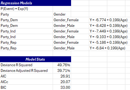
The model is given. If categorical predictors are present, then there is a model for each categorical level for each categorical predictor. The model statistics are then given. The deviance R2 and adjusted deviance R2 are given. The larger the percentages, the better the model is. Three others statistics are given:
- Akaike Information Criterion (AIC)
- AICc (Akaike’s Corrected Information Criterion)
- BIC (Bayesian Information Criterion)
These statistics are used to compare this model with other models. The smaller the values the better.
The Goodness of Fit table is then shown on the Summary worksheet.
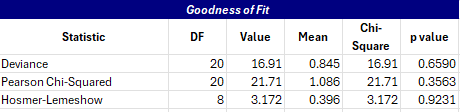
The value for the deviance is the error deviance from the Deviance Table above while the Pearson Chi-Squared value is the square of the Peason’s deviance (see below). The Hosmer-Lemeshow statistic is a goodness of fit test for logistic regression. The major reason for the Goodness of Fit table is to see how well the data fits the model. If there is a small p-value, then there is not a good fit.
The last portion of the Summary sheet is the Predict Results section.
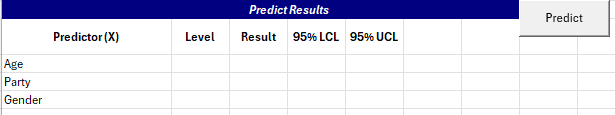
Enter values for the age, party and gender and then select Predict. The software will provide the result along with the 95% confidence limits.
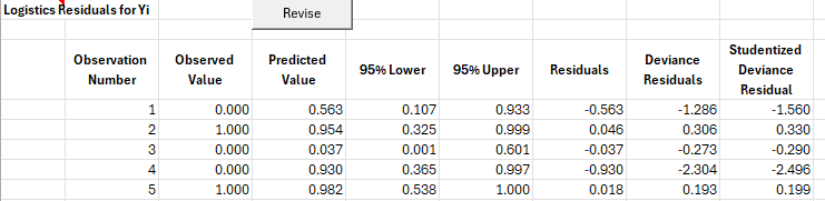
Residuals
The residuals worksheet contains the observation number, the observed values, predicted values, and the residuals using the options selected early or the defaults.
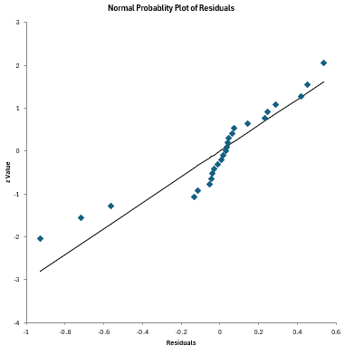
Regression Charts
There are two charts that are automatically created in this worksheet: a normal probability plot for the residuals and the predicted values versus observed values chart. The normal probability plot of the raw residuals is shown below. The residuals should fall around the straight line.
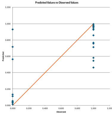
The predicted values versus observed values chart is shown below. A good model will have the points close to the line.
Additional charts are available from the “Revise” button on the residuals worksheet. See “Revising the Poisson Regression” below.
Revising the Binary Logistic Regression
SPC for Excel allows you to add additional charts on the Regression Charts worksheet, or to revise the regression by removing observations or removing variables. To access these options, select the “Revise” button on the residuals worksheet (see figure above). You will get the form below.
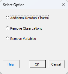
These three options are discussed below.
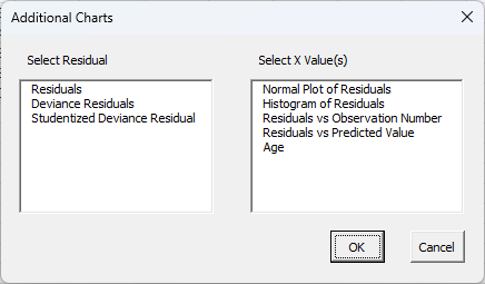
Additional Residual Charts
Selecting this option allows you to add additional charts via the form below. The residuals are listed on the left side (and will include leverage, etc. if those options were selected). You can select one type of residual. The possible X values are shown on the left-hand side. You may select multiple of these. Selecting OK will generate each chart selected and place them on the Regression Charts worksheet.
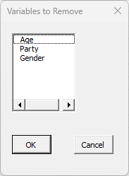
Remove Variables
If you select the remove variable option, you will see the input screen below. Select the variable(s) you want to remove. Select OK and a new regression will be run.
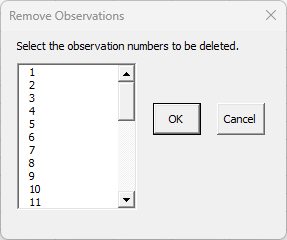
Remove Observations
I f you want to remove some of these observations, select the Remove Observations option. You will get a box that lists all the observations. Select the observation(s) you want to delete and then select OK. A new regression will be run.